
This post will compare the performance of the four pathfinding algorithms we coded in previous tutorials. We will look at each algorithm and find out which one is the fastest, which one generates the best path and which one explores the least nodes.
Algorithms
We first coded depth first search and watched it explore a node graph.

Then we coded breadth first search, and watched it explore a rectangular grid.

Next we coded greedy best first search, and watched it explore a hexagonal grid.

Finally we coded at a-star search, and watched it explore a triangular grid.

Hexagon Grid
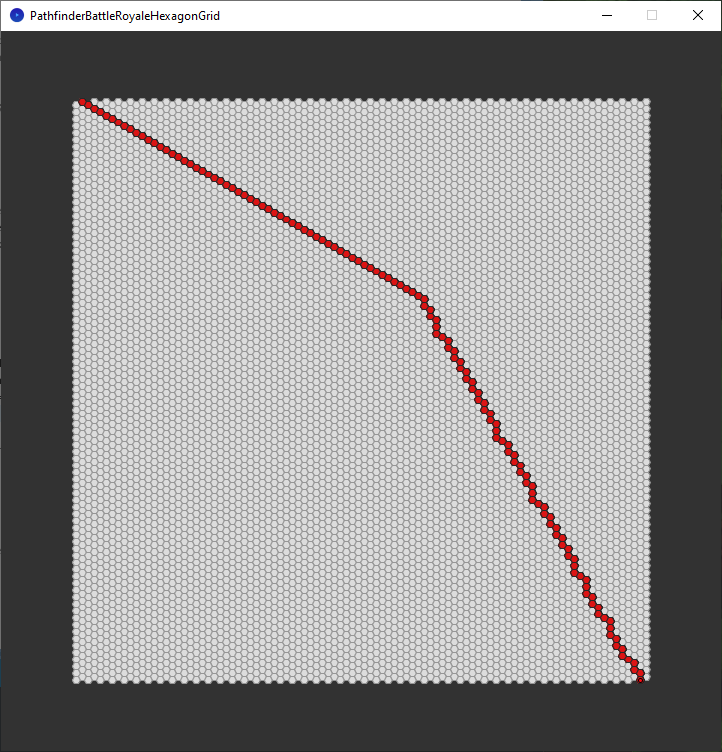
The test will be carried out on a large hexagon grid made up of 8,064 hexagon cells, some of which are walls. Only the cells which aren’t walls are connected as a node graph. The grid is made up of 48 columns by 168 rows.
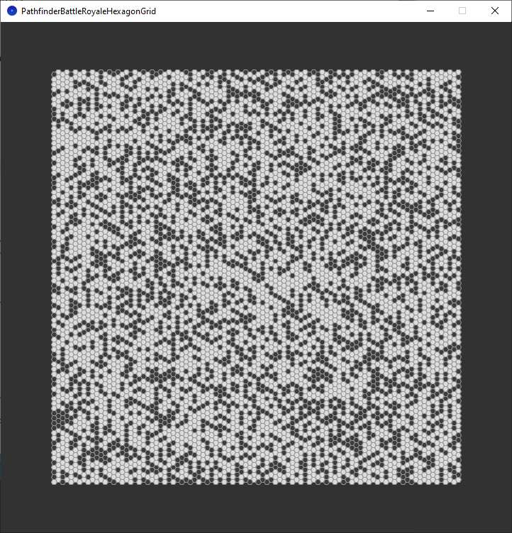
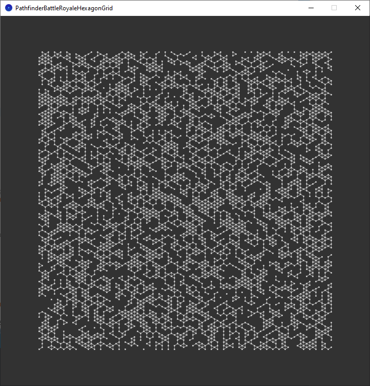
Here is what the node graph looks like.
Corner to Corner
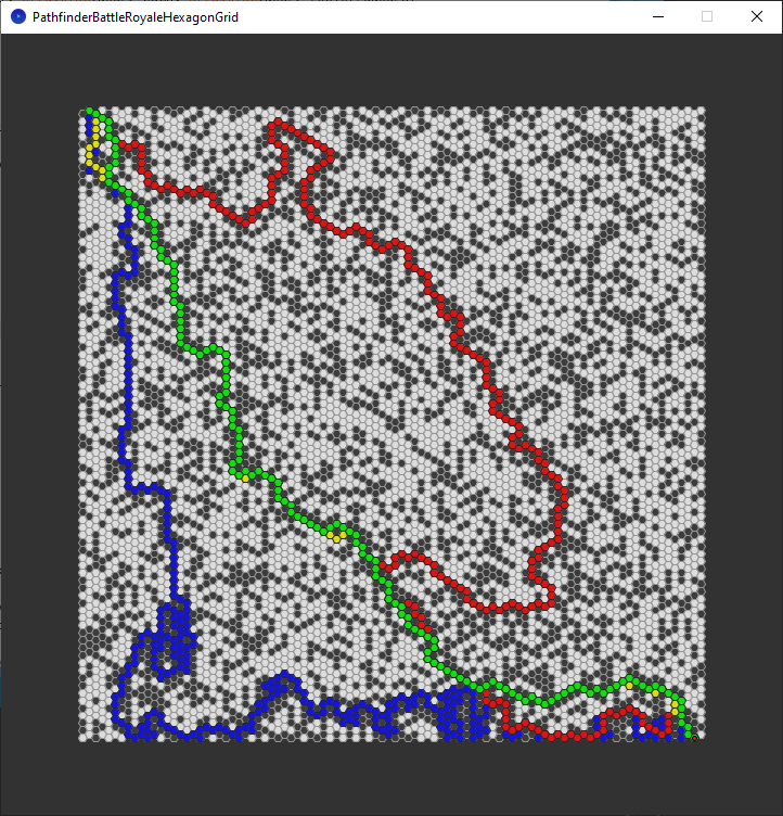
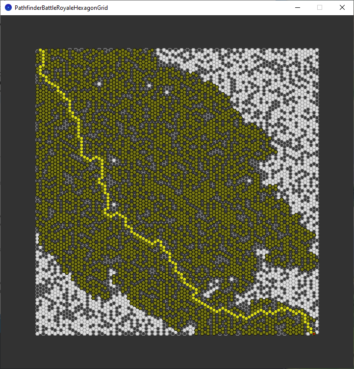
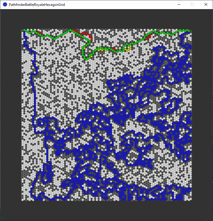
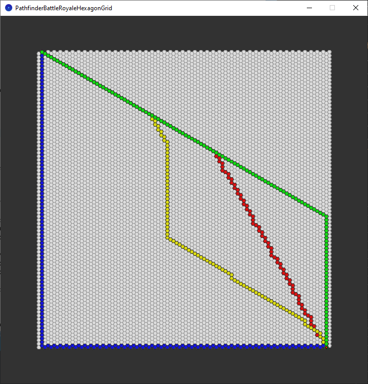
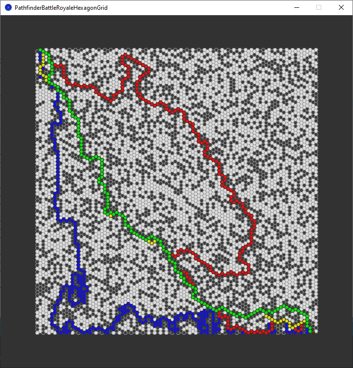
The four pathfinding algorithms start in the top left corner, and seek the goal in the bottom right corner.
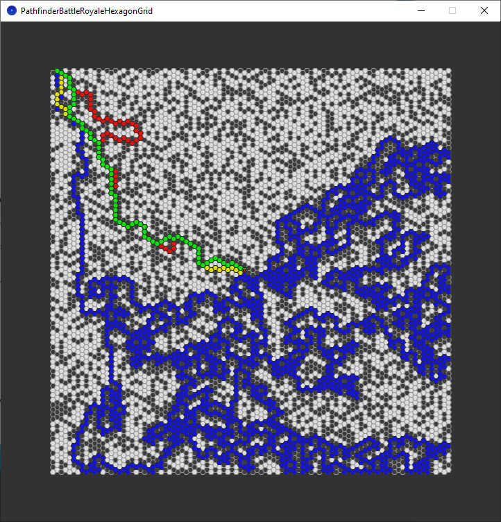
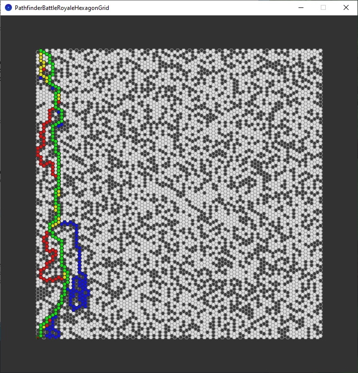
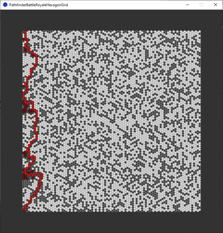
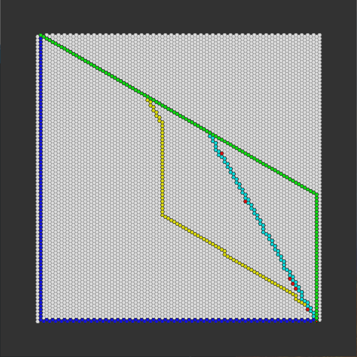
The chosen path each algorithm took. A-star (yellow) and breadth first search (green) take a path of the same length, but pick slightly different nodes. Greedy best first search (red) and depth first search (blue) picked routes which are far from perfect.
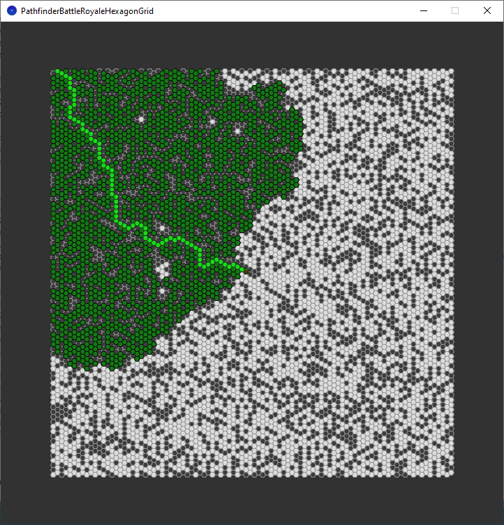
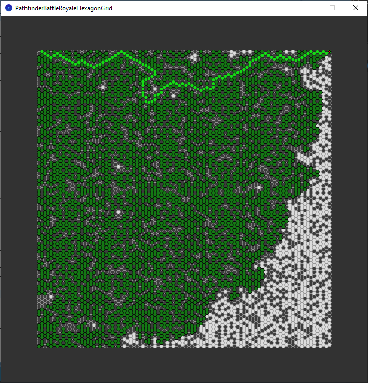
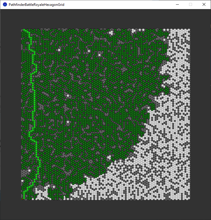
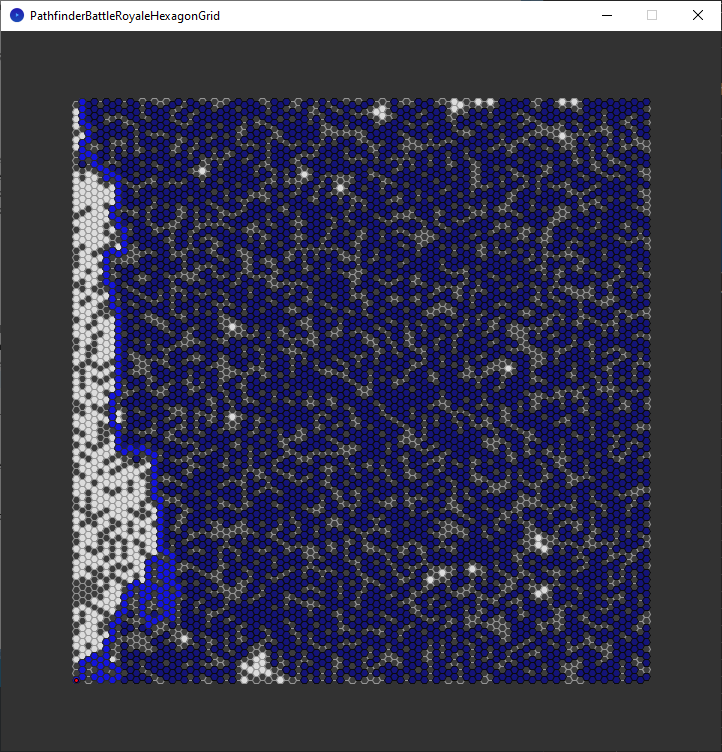
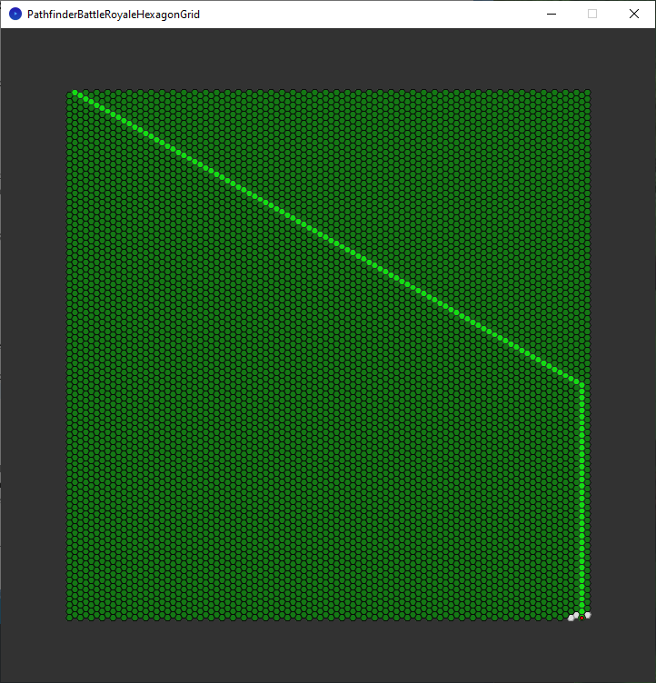
The nodes explored by breadth first search. This is almost the worst case scenario, since it explored almost every node except one (the one in blue).

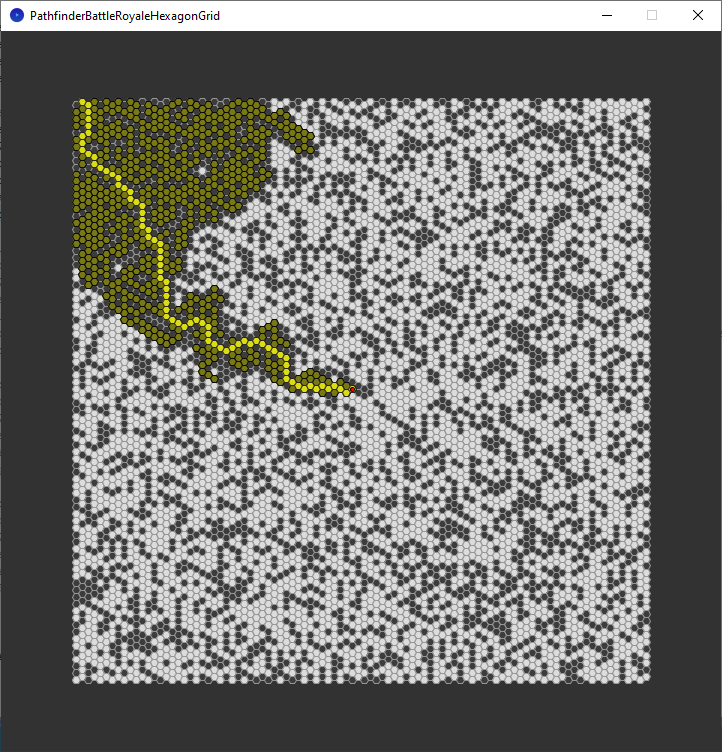
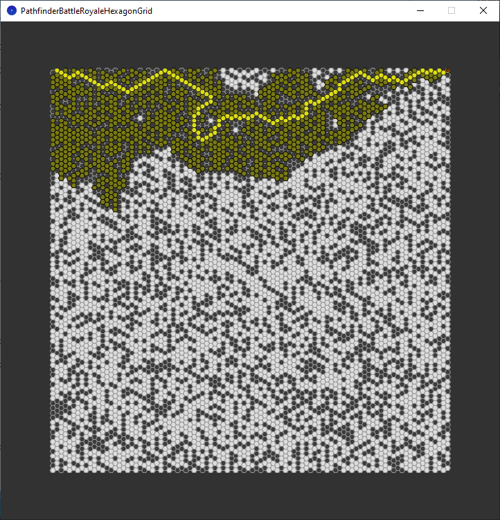
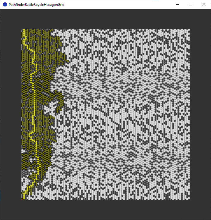
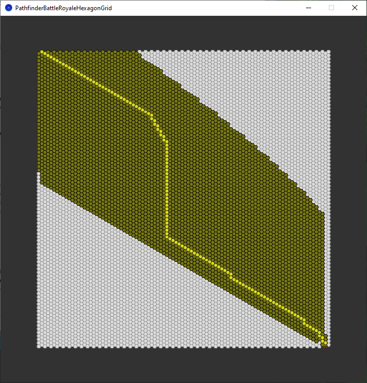
The nodes explored by a-star. Not as many as breadth first search, but still a large amount.
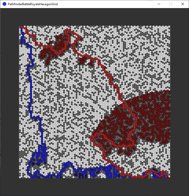
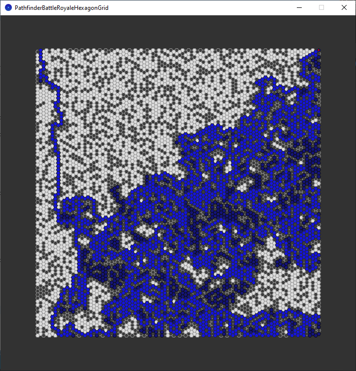
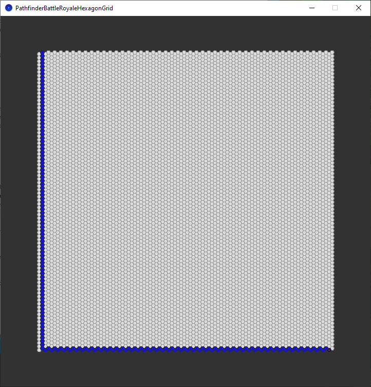
The nodes explored by both depth first search (in blue) and greedy best first search (in red). Both algorithms explored far less nodes than a-star and breadth first search.
The data from the test.
- Algorithm – The pathfinding algorithm.
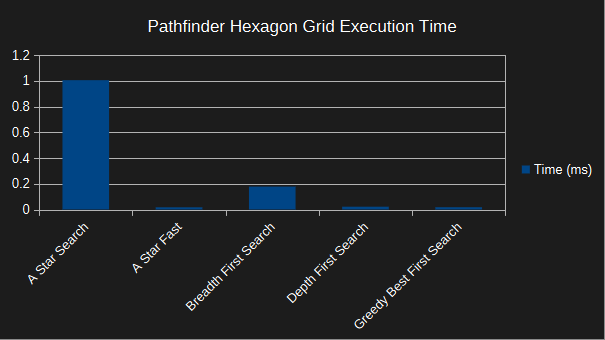
- Time (ms) – The time taken by each algorithm to calculate a path from the start point to the goal point in milliseconds.
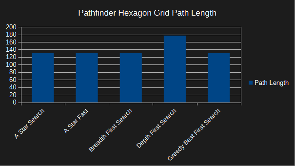
- Path Length – The length of the chosen path from the start point to the goal point.
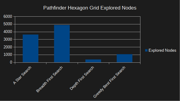
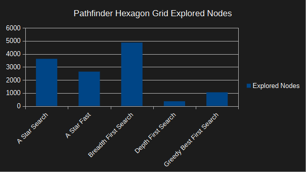
- Explored Nodes – The nodes explored by each algorithm.
| Algorithm | Time (ms) | Path Length | Explored Nodes |
| A Star Search | 9.1609 | 155 | 3623 |
| Breadth First Search | 1.6272 | 155 | 4875 |
| Depth First Search | 0.5373 | 325 | 362 |
| Greedy Best First Search | 0.5708 | 253 | 1051 |
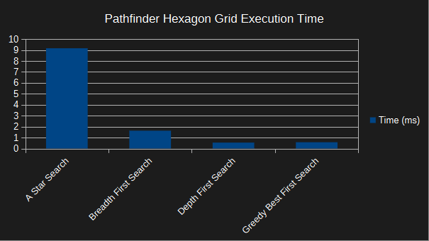
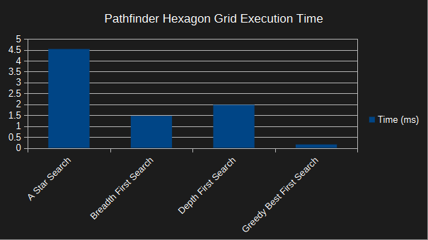
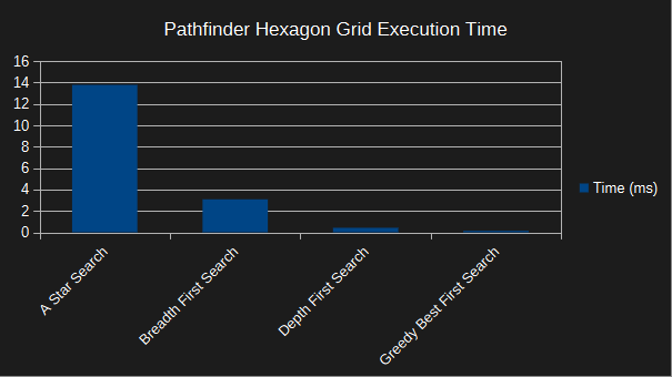
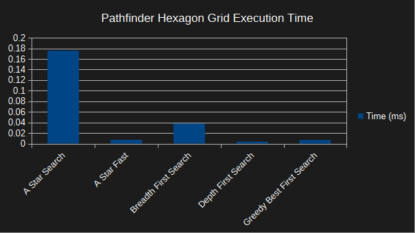
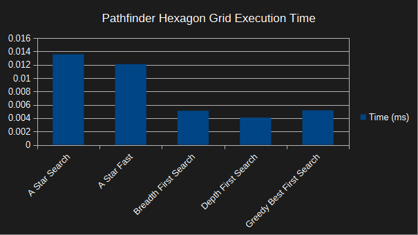
A chart showing the execution time of each pathfinding algorithm. As you can see, a-star is by far the slowest.
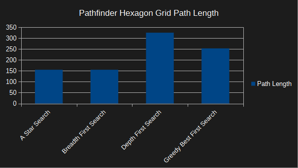
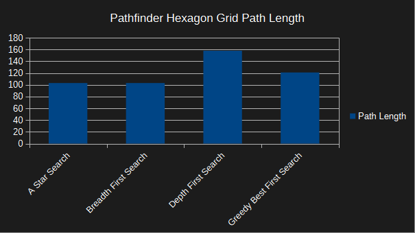
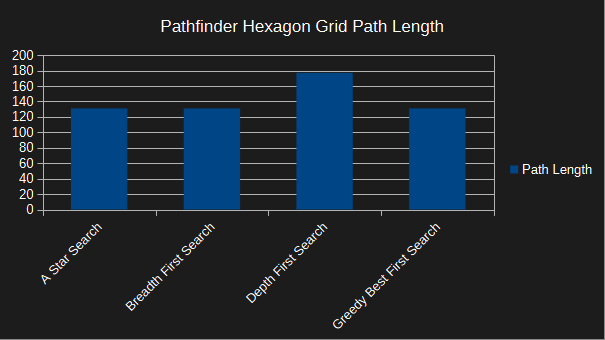
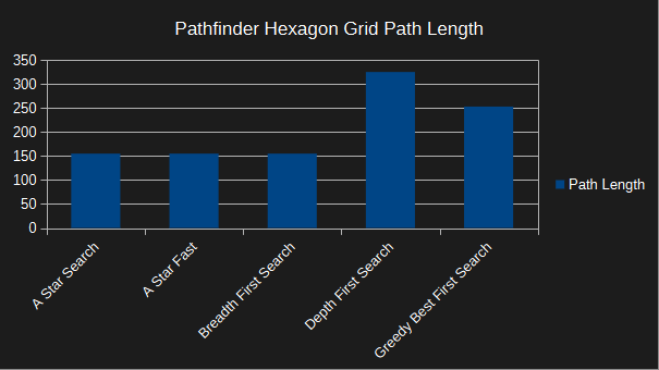
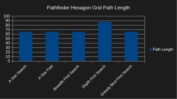
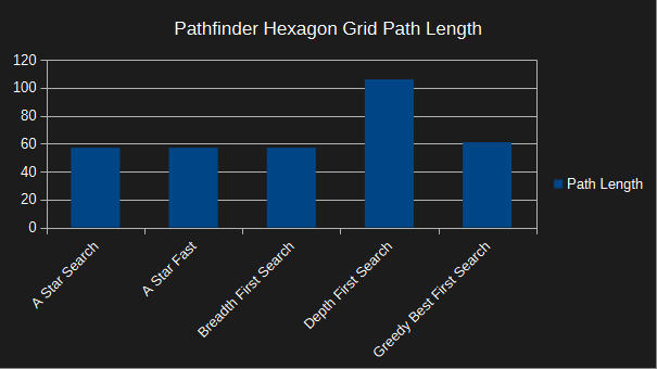
A chart showing the path length of each pathfinding algorithm. A-star and breadth first search both pick the shortest path in terms of the number of nodes. However they both pick slightly different paths. Depth first search picks the worst path.
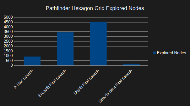
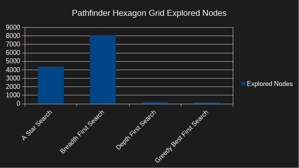
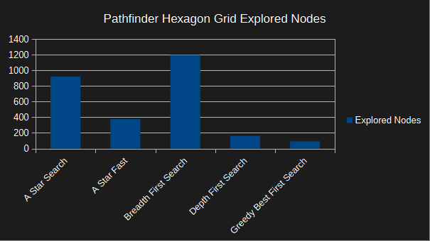
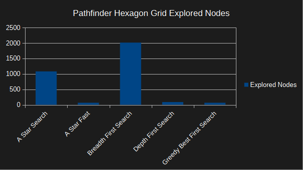
A chart showing the explored nodes of each pathfinding algorithm. Depth first search explores the least nodes. Breadth first search explores the most nodes.
Corner to Middle
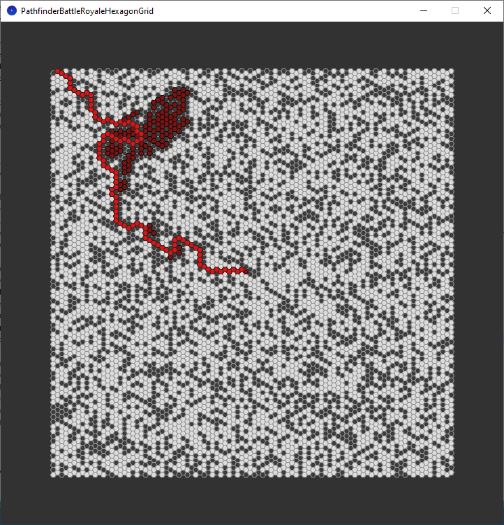
Next we will reuse the same hexagonal grid, and set the goal point to the middle of the grid.
The chosen path each algorithm took. A-star (yellow) and breadth first search (green) take a path of the same length, but pick slightly different nodes. Greedy best first search (red) picked a fairly good route, but depth first search (blue) picked a crazy long route!
The nodes explored by breadth first search. It explores a lot of nodes, before it finds the goal.
The nodes explored by a-star. It explores less nodes than breadth first search.
The nodes explored by depth first search. It explores a crazy number of nodes this time.
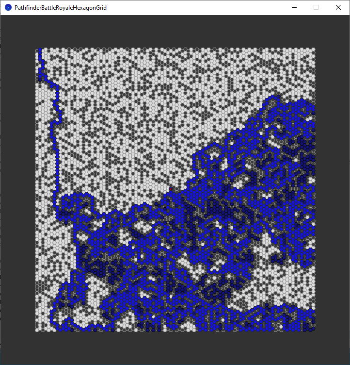
The nodes explored by greedy best first search. It explores a lot less nodes than the other algorithms.
The data from the test.
- Algorithm – The pathfinding algorithm.
- Time (ms) – The time taken by each algorithm to calculate a path from the start point to the goal point in milliseconds.
- Path Length – The length of the chosen path from the start point to the goal point.
- Explored Nodes – The nodes explored by each algorithm.
| Algorithm | Time (ms) | Path Length | Explored Nodes |
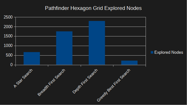
| A Star Search | 2.6094 | 76 | 662 |
| Breadth First Search | 0.9098 | 76 | 1749 |
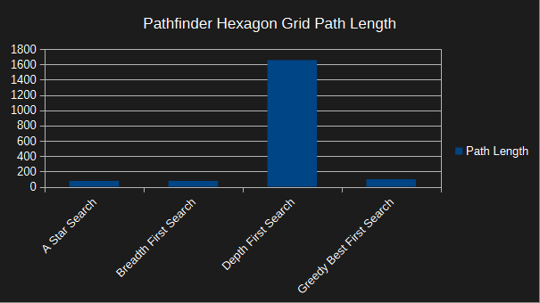
| Depth First Search | 1.7809 | 1657 | 2294 |
| Greedy Best First Search | 0.17 | 97 | 213 |
A chart showing the execution time of each pathfinding algorithm. As you can see, a-star is the slowest.

A chart showing the path length of each pathfinding algorithm. A-star and breadth first search both pick the shortest path in terms of the number of nodes. However they both pick slightly different paths. Depth first search picks the worst path.
A chart showing the explored nodes of each pathfinding algorithm. Depth first search explores the most nodes this time. Greedy best first search explores the least nodes.
Top Edge
Next we will reuse the same hexagonal grid, and set the goal point to the top right of the grid.
The chosen path each algorithm took. A-star (yellow), breadth first search (green) and greedy best first search (red) picked similar routes. Depth first search (blue) picked a crazy long route!
The nodes explored by breadth first search. It explores a lot of nodes, before it finds the goal.
The nodes explored by a-star. It explores less nodes than breadth first search.
The nodes explored by depth first search. It explores a crazy number of nodes.
The nodes explored by greedy best first search. It explores a lot less nodes than the other algorithms.

The data from the test.
- Algorithm – The pathfinding algorithm.
- Time (ms) – The time taken by each algorithm to calculate a path from the start point to the goal point in milliseconds.
- Path Length – The length of the chosen path from the start point to the goal point.
- Explored Nodes – The nodes explored by each algorithm.
| Algorithm | Time (ms) | Path Length | Explored Nodes |
| A Star Search | 4.5361 | 114 | 1011 |
| Breadth First Search | 1.4703 | 114 | 4068 |
| Depth First Search | 1.9762 | 1917 | 2619 |
| Greedy Best First Search | 0.1561 | 122 | 172 |
A chart showing the execution time of each pathfinding algorithm. As you can see, a-star is the slowest.
A chart showing the path length of each pathfinding algorithm. A-star and breadth first search both pick the shortest path in terms of the number of nodes. However they both pick slightly different paths. Depth first search picks the worst path.

A chart showing the explored nodes of each pathfinding algorithm. Breadth first search explores the most nodes. Greedy best first search explores the least nodes.

Left Edge
Next we will reuse the same hexagonal grid, and set the goal point to the bottom left of the grid.
The chosen path each algorithm took. A-star (yellow), breadth first search (green), greedy best first search (red) and depth first search (blue).
The nodes explored by breadth first search.
The nodes explored by a-star.
The nodes explored by depth first search.
The nodes explored by greedy best first search.
The data from the test.
- Algorithm – The pathfinding algorithm.
- Time (ms) – The time taken by each algorithm to calculate a path from the start point to the goal point in milliseconds.
- Path Length – The length of the chosen path from the start point to the goal point.
- Explored Nodes – The nodes explored by each algorithm.
| Algorithm | Time (ms) | Path Length | Explored Nodes |
| A Star Search | 3.5537 | 103 | 908 |
| Breadth First Search | 1.3273 | 103 | 3431 |
| Depth First Search | 2.7654 | 158 | 4527 |
| Greedy Best First Search | 0.1455 | 121 | 157 |
A chart showing the execution time of each pathfinding algorithm. As you can see, a-star is the slowest.

A chart showing the path length of each pathfinding algorithm. A-star and breadth first search both pick the shortest path in terms of the number of nodes. However they both pick slightly different paths. Depth first search picks the worst path.
A chart showing the explored nodes of each pathfinding algorithm. Depth first search explores the most nodes. Greedy best first search explores the least nodes.
No Walls
Next we will reuse the same hexagonal grid, and set the goal point to the bottom right corner of the grid. Except this time, the map will contain no walls!
The chosen path each algorithm took. A-star (yellow), breadth first search (green), greedy best first search (red) and depth first search (blue).
The nodes explored by breadth first search. As you can see, it explores almost every node.
The nodes explored by a-star. It explores quite a lot of nodes, but a lot less than breadth first search.
The nodes explored by depth first search. Depth first search gets lucky in this scenario and simply follows the edges of the map until it finds the goal.
The nodes explored by greedy best first search. It heads quickly to the goal point, as expected.
The data from the test.
- Algorithm – The pathfinding algorithm.
- Time (ms) – The time taken by each algorithm to calculate a path from the start point to the goal point in milliseconds.
- Path Length – The length of the chosen path from the start point to the goal point.
- Explored Nodes – The nodes explored by each algorithm.
| Algorithm | Time (ms) | Path Length | Explored Nodes |
| A Star Search | 13.7826 | 131 | 4345 |
| Breadth First Search | 3.0783 | 131 | 8061 |
| Depth First Search | 0.4169 | 177 | 177 |
| Greedy Best First Search | 0.1383 | 131 | 131 |
A chart showing the execution time of each pathfinding algorithm. As you can see, a-star is the slowest by a considerable margin. Probably because it is overwhelmed by adjacent nodes, looking for a shortest path, when there are actually many possibilities.
A chart showing the path length of each pathfinding algorithm. A-star, breadth first search and greedy best first search all pick the shortest path in terms of the number of nodes. However they all pick very different paths. Depth first search picks the worst path, as usual.
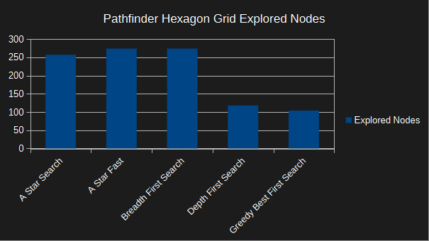
A chart showing the explored nodes of each pathfinding algorithm. Breadth first search explores almost all the nodes. Depth first search and greedy best first search explore the least nodes, and there path length is equal to the number of nodes they explore.
Conclusion
The worst algorithm by far is depth first search. The path it generates is to random to be useful for pathfinding from a start point to a goal point.
Greedy best first search is super quick, and usually explores a smaller number of nodes. However it’s path usually isn’t perfect, but it could be considered ‘good enough’, if speed is all you care about.
Breadth first search and A-Star search both calculate the shortest path, sometimes with slight differences in adjacent nodes. They can’t usually compete with greedy best first search in terms of execution time and the number of nodes explored. But they do generate the perfect path every time, which is what we want at the end of the day.
Breadth first search explores more nodes than A-Star search, however it’s execution time is usually a lot faster (as proven in the two examples above).
The reason it works better than A-Star in this case, is because we are using an unweighted graph. If we had to consider movement costs for a weighted graph, then A-Star should perform better. For example we could have mountain or swamp tiles which cost more time to cross.
The A-Star algorithm is also more complex. It needs to keep a container sorted, in this case we use a priority queue. It also needs to make sure there are no duplicates in the frontier. Although breadth first search handles duplicates in a different way, since it only explores each node once. Whilst A-Star can explore the same node multiple times.
Breadth first search could be slower in a very large map, where the goal is very far away. Greedy best first search would likely suffer more on a larger more complex map.
Overall breadth first search is the best pathfinding algorithm for unweighted graphs. It generates the best and shortest path in a good execution time.
Optimising A-Star
The current version of A-Star is based on the pseudocode from Wikipedia. We can clearly see that it works, since it always finds the shortest path. However it is not the fastest.
You can see the code for the full a-star search algorithm here.
Here are two optimisations which can greatly speed it up.
- Remove the duplicate check – allow duplicates in the frontier.
- Adjust the heuristic to prioritise the goal point.
So first off, we will remove the code which stops duplicates from being added to the frontier:
boolean duplicate = false;
for(Node f : frontier)
{
  if(f == node)
  {
    duplicate = true;
    break;
  }
}
if(!duplicate)
{
  frontier.add(node);
}
And replace it with this code, which will simply add the node to the frontier.
frontier.add(node);
Next we will create a multiplier variable at the start of the a-star function.
final float multiplier = 1.4;
We will use it when setting the goal score for the start node.
start.goalScore = Distance(start.position, goal.position) * multiplier;
And then later on, when we loop over the adjacent nodes.
node.goalScore = tentativeScore + Distance(node.position, goal.position) * multiplier;
So if we run this new code when the start point is the top left corner, and the goal point is the bottom right corner. Then we will get this:
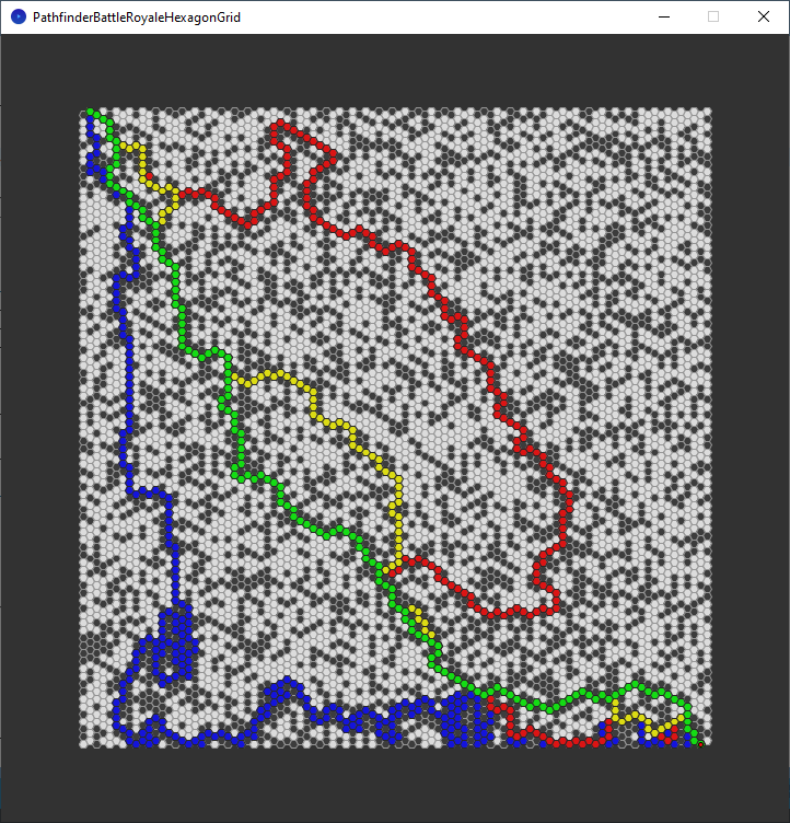
The chosen path each algorithm took. A-star (yellow) and breadth first search (green) take a path of the same length, but pick different nodes. Greedy best first search (red) and depth first search (blue) picked routes which are far from perfect.
The only difference I can see is that a-star takes a slightly different path in the bottom right corner to get to the goal. Notice how it diverges from breadth first searches path just before the goal point.
However the path length of both a-star and breadth first search is still the same.
The data from the test.
- Algorithm – The pathfinding algorithm.
- Time (ms) – The time taken by each algorithm to calculate a path from the start point to the goal point in milliseconds.
- Path Length – The length of the chosen path from the start point to the goal point.
- Explored Nodes – The nodes explored by each algorithm.
| Algorithm | Time (ms) | Path Length | Explored Nodes |
| A-Star | 9.1609 | 155 | 3623 |
| Optimised A-Star | 4.6102 | 155 | 2639 |
| Breadth First Search | 1.6272 | 155 | 4875 |
So as we can see, the optimised a-star is almost two times faster than the original a-star. The path length is also the same. The optimised a-star also explores less nodes.
However you need to be careful with the value you pick for the multiplier. The larger the multiplier, the less accurate the algorithm will become. We used 1.4 above, and that worked great. However if we use a multiplier of 2.0. Then we will get an a-star path which is longer and less accurate.
As you can see, the execution time is no quicker, the path length is now longer, but the number of explored nodes is a lot less.
| Algorithm | Time (ms) | Path Length | Explored Nodes |
| Optimised A-Star | 4.6401 | 164 | 1526 |
If you choose to use the multiplier, then it is likely you will need to adjust it for different maps.
Removing the duplicate check, so that duplicates are allowed into the frontier seems to have worked great for performance. However, I cannot guarantee that this won’t have side effects in certain scenarios.
So whichever algorithm you choose to use, make sure you thoroughly test it.
Full code for the optimised version of A-Star.
boolean AStarSearchFast(Node start, Node goal, ArrayList<Node> path, ArrayList<Node> exploredNodes, final float multiplier)
{
  path.clear();
  exploredNodes.clear();
  int moves = 0;

  start.startScore = 0.0f;
  start.goalScore = Distance(start.position, goal.position) * multiplier;

  PriorityQueue<Node> frontier = new PriorityQueue<Node>(10, new NodeGoalScoreComparator());
  frontier.add(start);
  Node current = null;
  float tentativeScore = 0;
  while(!frontier.isEmpty())
  {
    ++moves;
    current = frontier.poll();
    exploredNodes.add(current);

    if(current == goal)
    {
      println("Goal has been found in " + moves + " moves");
      while(current != null)
      {
        path.add(current);
        current = current.parent;
      }
      Collections.reverse(path);
      return true;
    }

    for(Node node : current.adjacentNodes)
    {
      tentativeScore = current.startScore + Distance(current.position, node.position);
      if (tentativeScore < node.startScore)
      {
        // This path to neighbour is better than any previous one. Record it!
        node.parent = current;

        node.startScore = tentativeScore;
        node.goalScore = tentativeScore + Distance(node.position, goal.position) * multiplier;

        frontier.add(node);
      }
    }
  }

  println("Failed to find the goal in", moves, "moves");
  return false;
}
Improved Testing
Running the tests in the Processing ‘setup’ function has caused some slowdowns. It turns out the algorithms are a lot faster when ran later, when the code has been warmed up.
To improve the tests I am now running each algorithm 100 times, then taking the average like so:
  time = 0;
  for(int i=0; i<total; ++i)
  {
    ResetAllNodes();
    timer.Start();
    AStarSearch(startNode, goalNode, aStarPathRenderer.pathList, aStarPathRenderer.exploredNodes);
    time += timer.GetMillis();
  }
  println(aStarPathRenderer.name, time / (double)total, aStarPathRenderer.pathList.size(), aStarPathRenderer.exploredNodes.size());
However, the tests are also slow when ran for the first time, so I ran all the tests 10 times by pressing a button. Every button press executes a new test. Then I use the data from the last test. So this means that each algorithm is ran 1000 times.
  if(key == 'r' || key == 'R')
  {
    RunPathfinderTest();
  }
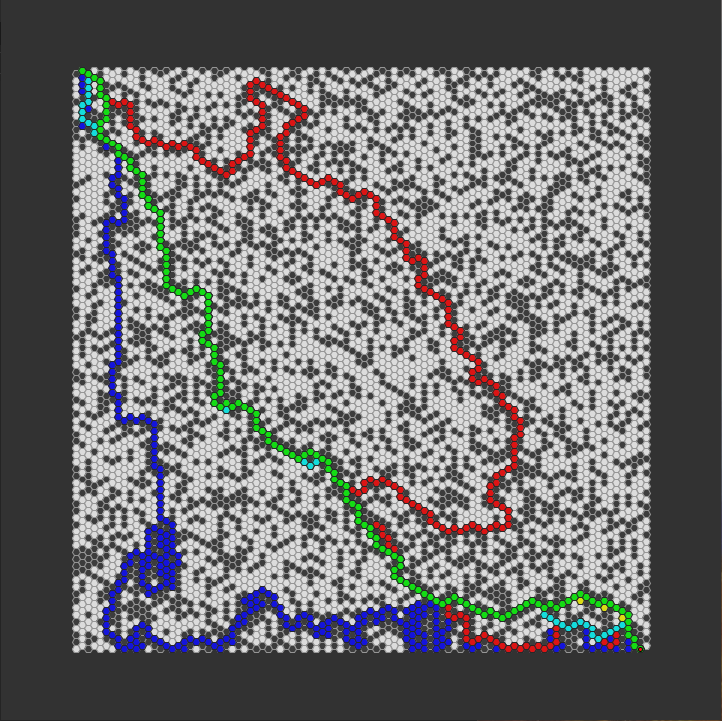
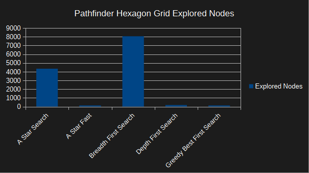
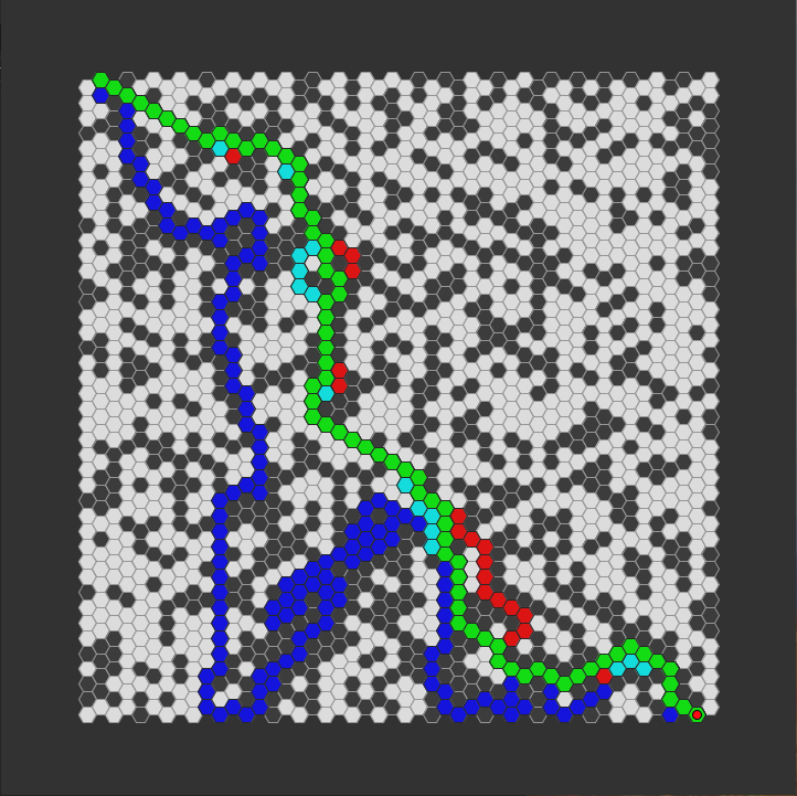
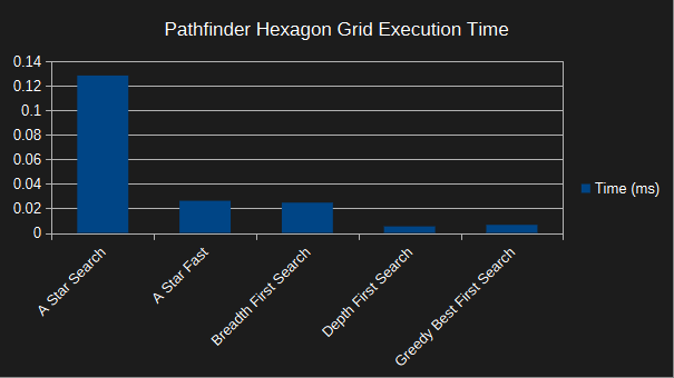
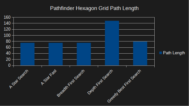
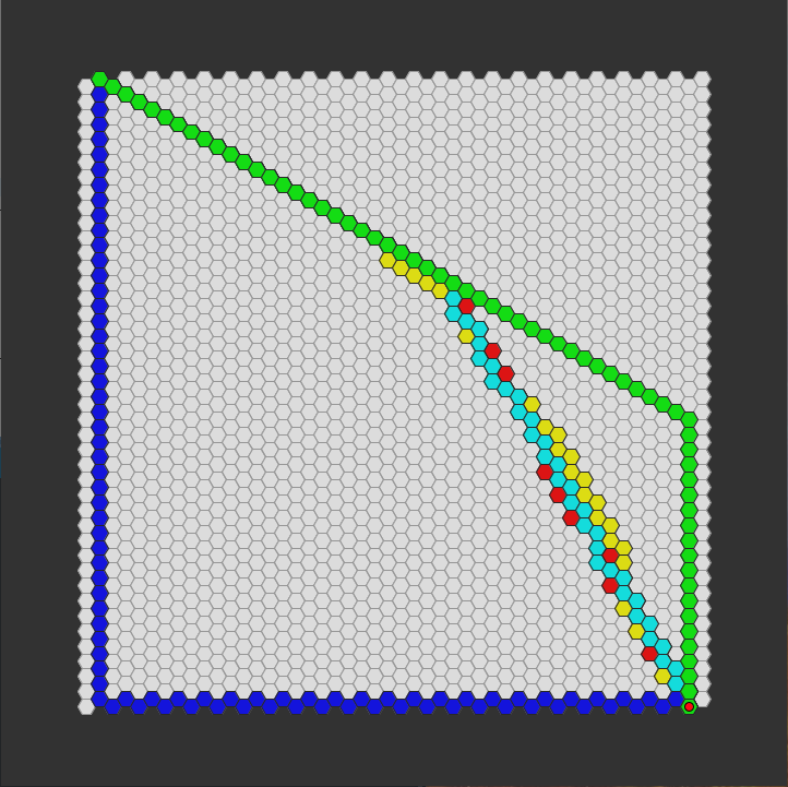
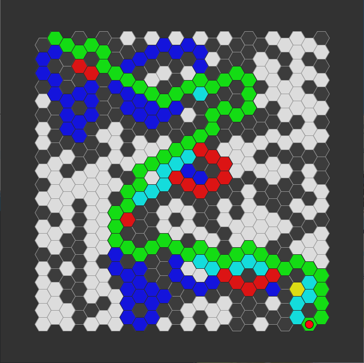
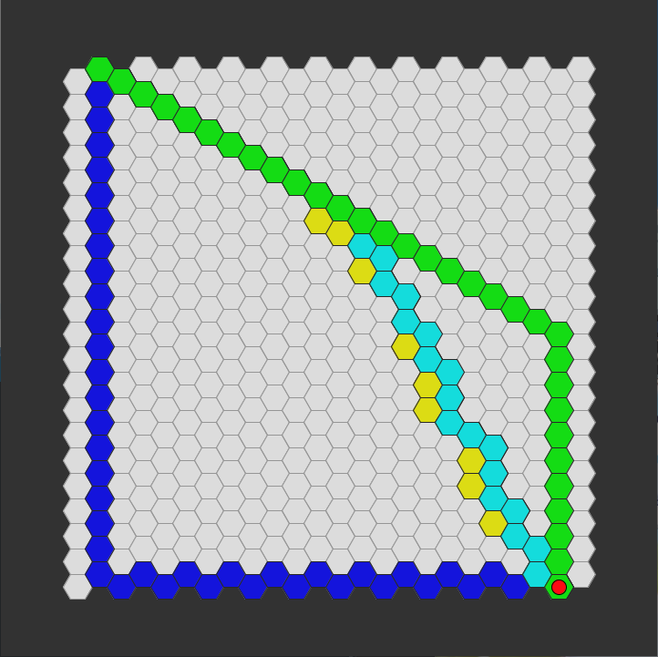
So if the corner to corner map is used again, but with the fast A-Star added, then the paths look like this:
The chosen path each algorithm took. A-Star (yellow), fast A-Star (Cyan), breadth first search (green), greedy best first search (red) and depth first search (blue).
Here is the data from the first test.
| Algorithm | Time (ms) | Path Length | Explored Nodes |
| A-Star | 1.675204980969429 | 155 | 3623 |
| Fast A-Star | 0.5141060307621956 | 155 | 2639 |
| Breadth First Search | 0.3697878807783127 | 155 | 4875 |
| Depth First Search | 0.13196402050554754 | 325 | 362 |
| Greedy Best First Search | 0.20337198927998543 | 253 | 1051 |
And the data from the tenth test:
| Algorithm | Time (ms) | Path Length | Explored Nodes |
| A-Star | 0.656989073157311 | 155 | 3623 |
| Fast A-Star | 0.262296930849552 | 155 | 2639 |
| Breadth First Search | 0.151341029256582 | 155 | 4875 |
| Depth First Search | 0.0153920302167535 | 325 | 362 |
| Greedy Best First Search | 0.0980640694499016 | 253 | 1051 |
Notice how the algorithms are much slower on the first test, even though this is ran outside of the Processing ‘setup’ function at a time of my choosing when I press a button. Also tests two to nine are similar to ten, and not to one. The first test is very much an anomaly.
However when the original A-Star algorithm was ran in the setup function, it took ‘9.1609’ milliseconds. Which is a massive difference.
I currently do not know why the A-Star algorithm takes ‘1.675204980969429’ milliseconds in the first test, and only ‘0.656989073157311’ milliseconds in the tenth test.
I would guess it could have something to do with one or all of the following:
- Processing is doing something in the background
- Caching
- Automatic garbage collection
In relation to caching, the majority of the variables and containers are created and destroyed within each algorithms function. The nodes are reset before each test. The path list and explored nodes list have there capacities set to the number of nodes in the grid.
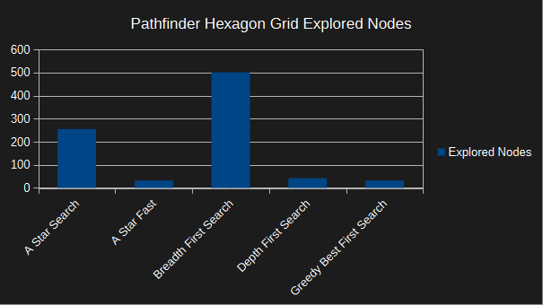
Here are the charts with the new data.

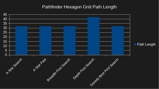
So no new changes overall despite the speed increase. The breadth first search algorithm is still outperforming both a-star algorithms.
Now lets take a look at the same map, but without the walls.
| Algorithm | Time (ms) | Path Length | Explored Nodes |
| A-Star | 1.00576806306839 | 131 | 4345 |
| Fast A-Star | 0.01687483988702 | 131 | 131 |
| Breadth First Search | 0.178006018400192 | 131 | 8061 |
| Depth First Search | 0.0216510004643351 | 177 | 177 |
| Greedy Best First Search | 0.017456190418452 | 131 | 131 |
So at last we have a case where the optimised version of A-Star beats breadth first search. This is down to A-Star following the path of greedy best first search. Notice how the number of explored nodes are the same as the path length. This is why the multiplier is important. However, this was not the case when we had a map with walls.
Small Map
Next we will look at a map which is half the size of the one we used previously.
| Algorithm | Time (ms) | Path Length | Explored Nodes |
| A-Star | 0.128427950441837 | 75 | 920 |
| Fast A-Star | 0.0261839399300516 | 75 | 376 |
| Breadth First Search | 0.0246970299445093 | 75 | 1196 |
| Depth First Search | 0.00530396993272007 | 148 | 162 |
| Greedy Best First Search | 0.00656900998204947 | 79 | 92 |
Looks like breadth first search is faster than A-Star, but only by a sliver.
Now we will look at the same map but without the walls.
| Algorithm | Time (ms) | Path Length | Explored Nodes |
| A-Star | 0.175745959877968 | 65 | 1081 |
| Fast A-Star | 0.00719500006642193 | 65 | 65 |
| Breadth First Search | 0.0379140102863312 | 65 | 2013 |
| Depth First Search | 0.00377391001442447 | 87 | 87 |
| Greedy Best First Search | 0.00682299995329231 | 65 | 65 |
The optimised version of A-Star is faster than breadth first search.
Very Small Map
Next we will look at one more map, which is half the size of the small map.
| Algorithm | Time (ms) | Path Length | Explored Nodes |
| A-Star | 0.0135750101227313 | 57 | 257 |
| Fast A-Star | 0.0121070099249482 | 57 | 274 |
| Breadth First Search | 0.00511400006711483 | 57 | 274 |
| Depth First Search | 0.00408098998013884 | 106 | 118 |
| Greedy Best First Search | 0.00517000005114824 | 61 | 104 |
Interestingly the optimised version of A-Star is a lot slower than breadth first search this time. I would guess the wall placement has had a significant effect.
Now lets look at the same map, but without the walls.
| Algorithm | Time (ms) | Path Length | Explored Nodes |
| A-Star | 0.0230150301381946 | 32 | 255 |
| Fast A-Star | 0.00444602996110916 | 32 | 32 |
| Breadth First Search | 0.0110369900520891 | 32 | 501 |
| Depth First Search | 0.00208800998632796 | 42 | 42 |
| Greedy Best First Search | 0.00278704997850582 | 32 | 32 |

Again we have another case where the optimised A-Star algorithm is faster than breadth first search. But of course on an open map without walls, we don’t even need pathfinding algorithms.
Conclusion Two
Overall it seems like breadth first search is still the best choice overall for an unweighted graph, since it is consistent. If you want to use A-Star, then you will need to play with the multiplier to balance speed with the shortest path.
